2 Lab 1 - 26/09/2024

In this lab we will learn the basic commands for programming with R. We will work in RStudio.

To start, place your cursor in the Console (bottom-left on RStudio) and type the following code or any other mathematical operation:

5+4

[1] 9

R can work like a calculator and you can compute whatever quantity you need. The point is that if you close RStudio, you will lose all your code. To avoid this, I suggest to use scripts (i.e. text files where you can write and run your code). To open a new script, we can use the RStudio menu: File - New File - RScript. Write all your code in your script and use ctrl/cmd + enter to run the code in the Console. Save the script by using the menu: File - Save as…. The extension of a script is .R (choose the name you prefer). In the future you will be able to open your script with RStudio without losing anything.

2.1 Built-in functions

Before starting using a function, it is good pratice to visualise the help page (by running ?nameofthefunction), in order to understand how the function is defined and which are its arguments and the default settings.

To run a function (and get the results) type the name of the function followed by round parentheses, inside which you specify the arguments of the functions (the inputs).

For example to compute the logarithm of a number the function log is used. Its help page can be obtained by

#?log

Note that the function is characterized by two arguments: x, that is the number or vector for which the log is computed and base, that is the base of the log function. Let’s compute the log as follows:

log(x = 5 , base = 10) #log of 5 with base 10

[1] 0.69897

If we omit to specify the base R runs a natural logarithm.

log(x = 5) #natural log of 5

[1] 1.609438

Argument names can be omitted. In this case it is very important to be careful about the order of the arguments passed to the function (the order is given by the function definition, check the help).

log(5, 10)

[1] 0.69897

log(10, 5) #warning: this is log of 10 with base 5

[1] 1.430677

2.2 Objects and vectors

In R it is possible to create objects by using the assignment operator = (it is also possible to use <-). As argument name you can choose any name you prefer; however, it’s better to use short and meaningful names. The following code assigns the number -1.5 to the object named x (have a look to the top right panel!):

x = -1.5

We can also create objects that contains vectors. A vector of number is created using the c function (concatenate). For example the following code is used to create a vector with 4 numbers. The vector is saved in an object named y:

y = c(-1.5, 99, log(15), 6.7)

To visualize the values of y just run the object name (remember that R is case-sensitive so that y is different from Y):

[1] -1.50000 99.00000  2.70805  6.70000

The vector length is given by

length(y)

[1] 4

It is possible to compute operations with vector. For example, the following code add 5 to all the elements of y. Here, we are not going to modify the vector y, that remains the same.

y + 5

[1]   3.50000 104.00000   7.70805  11.70000

[1] -1.50000 99.00000  2.70805  6.70000

If we want to rewrite the vector y, we have to use the assignment operator.

y = y + 5 #rewriting the vector y
y

[1]   3.50000 104.00000   7.70805  11.70000

Note that R executes operations with vector element-wise (element by element singularly). The same element-wise approach is adopted also for computing operations involving two vectors of the same length:

# create another object z
z = c(6.89, -10, 5.5, sqrt(log(5))) 
z

[1]   6.890000 -10.000000   5.500000   1.268636

# operations with 2 vectors
y - z

[1]  -3.39000 114.00000   2.20805  10.43136

To select elements from a vector we use squared parentheses. For example, to retrieve the second element the following code is used. we need to specify inside the parentheses the position of the element to be select:

y[2]

[1] 104

To select more than one element, a vector of positions is provided:

y[c(1,4)] #select the first and forth element

[1]  3.5 11.7

If you need to select the first three element of y you can proceed as follows:

y[c(1,2,3)]

[1]   3.50000 104.00000   7.70805

or by using the following shorter code where 1:3 generates a regular sequence of integers from 1 to 3:

1:3

[1] 1 2 3

y[1:3]

[1]   3.50000 104.00000   7.70805

To replace values (after having selected them) we use the assignment operator =:

# select the second element and replace it with 4
y[2] = 4
y

[1]  3.50000  4.00000  7.70805 11.70000

It is also possible to summarize the values in a vector by using summary statistics function such as the sum or the mean applied to y or any function of it:

sum(y) #sum of the elements of y

[1] 26.90805

mean(y) #mean of the values of y

[1] 6.727013

sum(y) / length(y) #another way for computing the mean

[1] 6.727013

mean((y^3)+4) #first the operation ^3+4 is computed and then the sum

[1] 545.6136

There are also other summary functions such as, for example, median, quantile, min and max.

It is also possible to compute logical operation whose result is TRUE if the condition is met or FALSE otherwise. For example:

z >= 0

[1]  TRUE FALSE  TRUE  TRUE

gives a vector of TRUE/FALSE according to the condition ‘bigger than or equal to 5’ applied to each element of y. Summary statistics can be applied also to vector of logical values, in this case TRUE is considered as 1 and FALSE as 0.

sum(z >= 0) #number of values that met the condition (z>= 0)

[1] 3

mean(z >= 0) #proportion  of values  that met the condition (z>= 0)

[1] 0.75

mean(z >= 0)*100 #percentage of values that met the condition (z>= 0)

[1] 75

#comment: 75% of the observation are bigger or equal to 0.

The following table lists all the logical operators available in R.

Operator in R	Description
<= >=	lower/bigger than or equal
< >	lower/bigger
==	exactly equal to
!=	different from
&	intersection (and)
`\|` (vertical bar)	union (or)

By using logical operator it is possible to select/replace elements in a vector by setting a condition. In this case it is not necessary to specify the positions in the vector of the elements to be selected/replaced. R will consider only the elements for which the condition is met:

# substitute the positive numbers of z with 0
z[z > 0] = 0
z

[1]   0 -10   0   0

Let’s create now a new vector object called z2 which contains all the element of z different from -10. In this case the condition which is tested is z != -10 which returns the following logical vector

z != -10

[1]  TRUE FALSE  TRUE  TRUE

! (z == -10) #another way to identify all the value different form -10

[1]  TRUE FALSE  TRUE  TRUE

Finally, we can do the selection and create z2:

z[ z != -10] #we select all the value that met the condition

[1] 0 0 0

z2 = z[ z != -10] #we assign those values into a new vector (z2). 
z2

[1] 0 0 0

2.3 (Pseudo) Random number simulation

In Section @ref(objectsandvectors) we have already introduced the concept of numerical vector.

An example of random generation is given by the random experiment that consists in tossing a coin five times (T=tail, H=head). One possible outcome is {T, H, H, T, T}, while {H, H, H, T, H} is another possible random sequence. All the random sequence of Head and Tail are simulated from the distribution which assigns probability 0.5 to Head and probability 0.5 to Tail.

The function sample can be used to perform the coin random experiment (see ?sample). With the following code we toss the coin 10 time (two possible outcomes: head and tail) and save the (random) output in a vector named coin which is a vector of strings (character):

?sample
coin = sample(x = c("head", "tail"), size = 10, replace = TRUE)
coin

 [1] "head" "head" "tail" "tail" "tail" "head" "head" "tail" "head" "head"

class(coin)

[1] "character"

As the procedure is random every time you run sample you will get a different output.

Given the vector coin it is possible to compute how many times we got head/tail and to plot this frequency distribution:

table(coin) # frequency distribution

coin
head tail 
   6    4

barplot(table(coin)) #plot the frequency distribution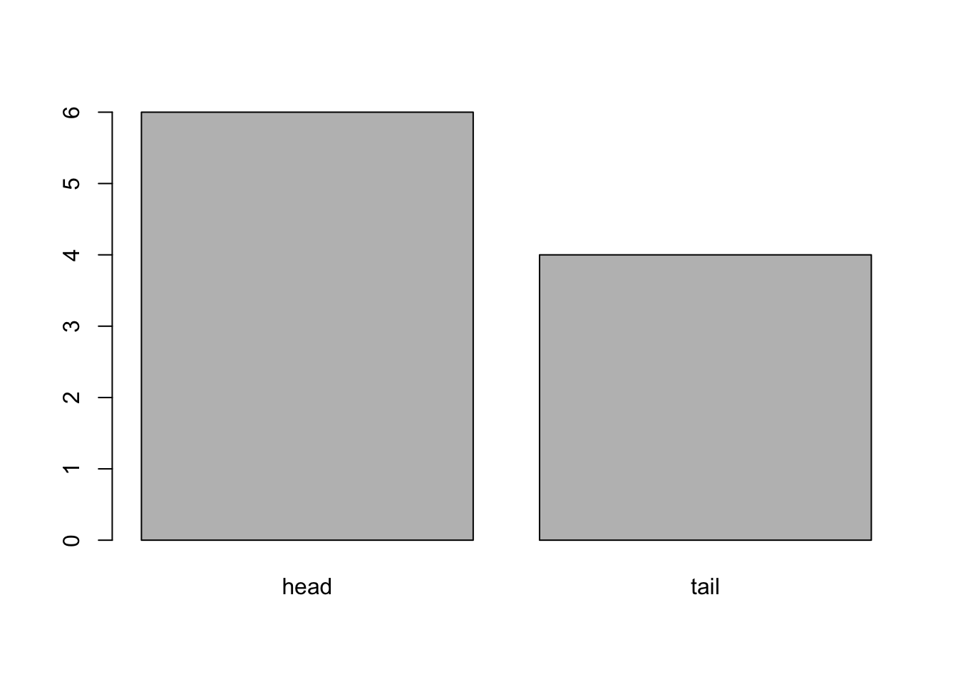

We will now create a vector containing 10 numbers simulated from the continuous Uniform distribution (see here). We consider an Uniform(0,1) which can take all the real values between 0 and 1. In this case we resort to a specific R function named runif (r... stands for random), see ?runif. For simulating randomly 10 numbers from the Uniform distribution defined with 0 and 1 (default values), we use the following code:

runif(10)

 [1] 0.22242096 0.85733920 0.24010865 0.20746429 0.04722797 0.36018585
 [7] 0.40503215 0.76297528 0.51169527 0.53966016

This code returns 10 different number every time you run it. In order to get the same data, for reproducibility purposes, it is necessary to set the seed (i.e. to set the starting point of the algorithm which generates the random numbers). To do this the set.seed function is used; it takes as input an integer positive number (55 in the following example):

set.seed(55)
a = runif(10)
a

 [1] 0.54781352 0.21815968 0.03496399 0.79154929 0.56024208 0.07422517
 [7] 0.13152294 0.29412388 0.50076126 0.08832446

class(a)

[1] "numeric"

The 10 numbers are saved in an object named a which is a numerical vector. By setting the seed we are able to reproduce always the same sequence of random numbers (which is the same for all of us). In this case the numbers are said to be pseudo-random (and not fully random as they can be reproduced).

The 10 values can be plotted by using the following code that returns an histogram:

hist(a)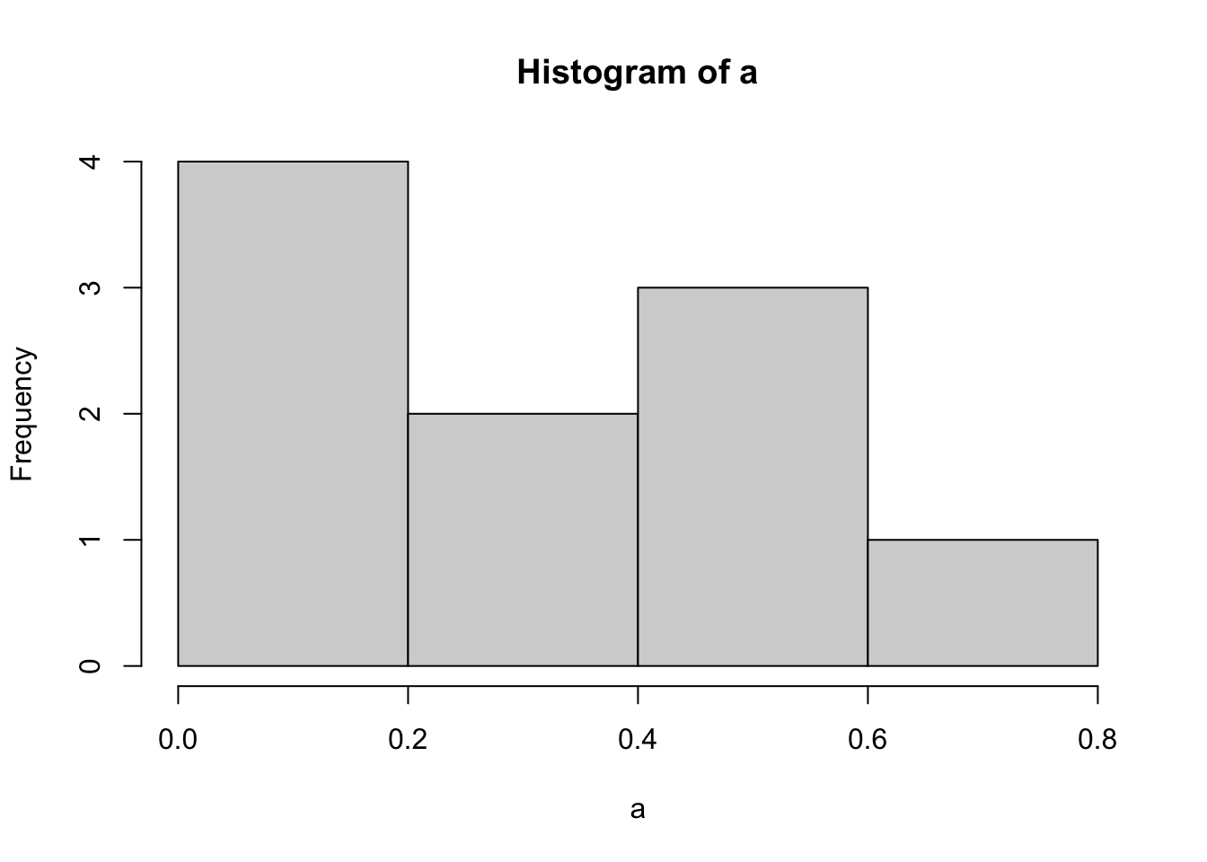

It is also possible to reduce the number of decimals by using the function round (see ?round). For example, we decide to have the number in a with 2 decimals:

z = round(a, 2)
z

 [1] 0.55 0.22 0.03 0.79 0.56 0.07 0.13 0.29 0.50 0.09

To check the type of object the function class can be used:

class(z)

[1] "numeric"

In this case z is a vector of real numbers (numeric).

Let’s assume now to combine coin and a by concatenating (with the c function) the two vectors:

w = c(coin, a)
w

 [1] "head"               "head"               "tail"              
 [4] "tail"               "tail"               "head"              
 [7] "head"               "tail"               "head"              
[10] "head"               "0.547813516110182"  "0.218159678624943" 
[13] "0.0349639947526157" "0.791549294022843"  "0.560242076171562" 
[16] "0.074225174030289"  "0.131522935815156"  "0.294123877771199" 
[19] "0.500761263305321"  "0.088324457872659"

class(w)

[1] "character"

Note that w is a vector of text strings (character) and also the numbers have been forced to text (we can observe it because numeric values are in quotes). This is not happening if we combine two numerical vectors as a and z:

p = c(a, z)
p

 [1] 0.54781352 0.21815968 0.03496399 0.79154929 0.56024208 0.07422517
 [7] 0.13152294 0.29412388 0.50076126 0.08832446 0.55000000 0.22000000
[13] 0.03000000 0.79000000 0.56000000 0.07000000 0.13000000 0.29000000
[19] 0.50000000 0.09000000

class(p)

[1] "numeric"

length(p) #check how many elements in p

[1] 20

2.4 Normal distribution

The Normal distribution is the most known and used continuous random variable (see here). The function for simulating values from the Normal distribution is rnorm (see ?rnorm).

First, we compute 100 values from the Normal distribution with mean 5 and variance 4.

set.seed(55)
mynorm = rnorm(100, mean = 5, sd = sqrt(4))

We then plot the simulated data and compute some (empirical) summary statistics:

hist(mynorm)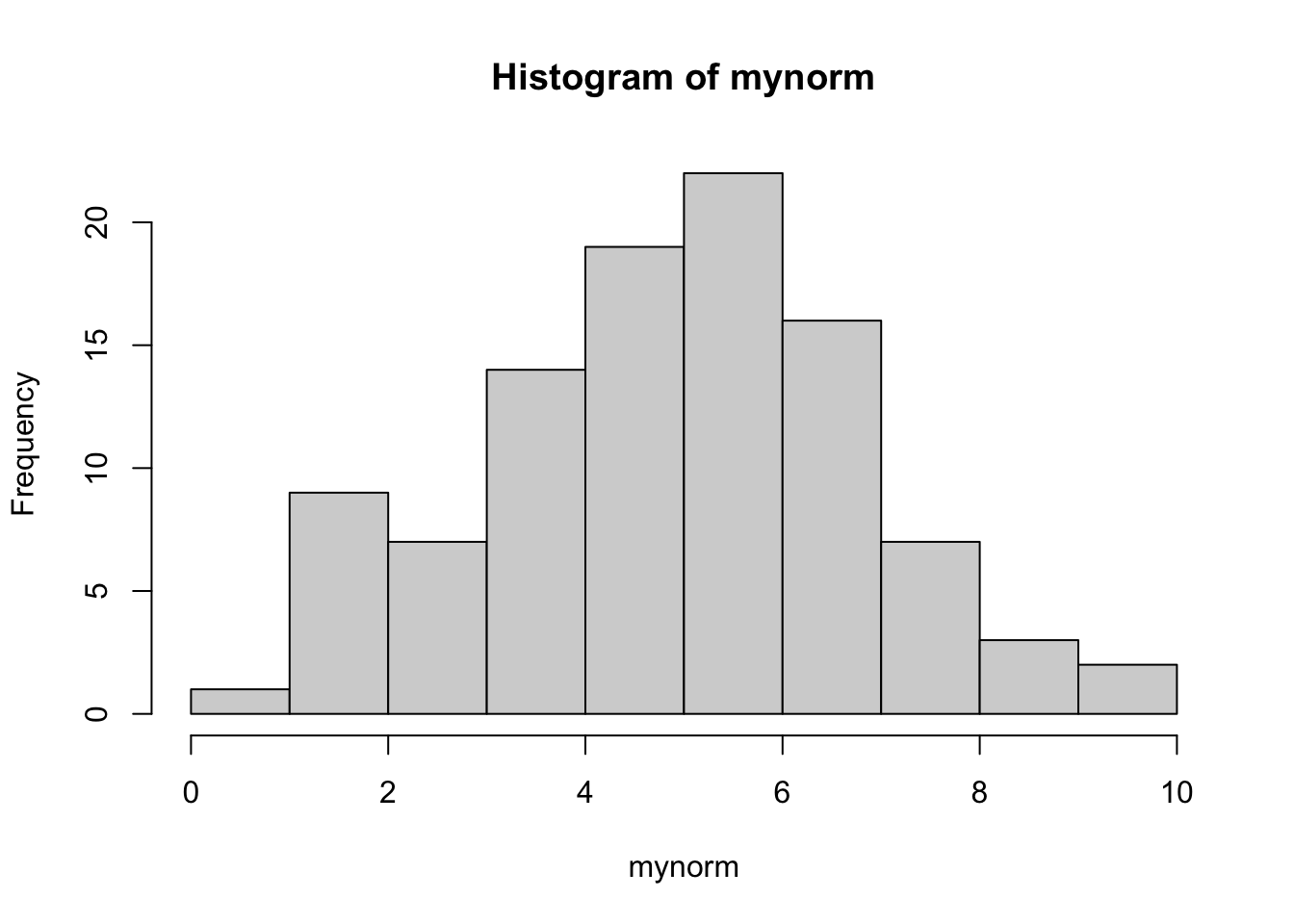

We sample here below 1000 values from the same Normal distribution.

set.seed(55)
mynorm = rnorm(1000, mean = 5, sd = sqrt(4))

We then plot the simulated data and compute some (empirical) summary statistics:

hist(mynorm)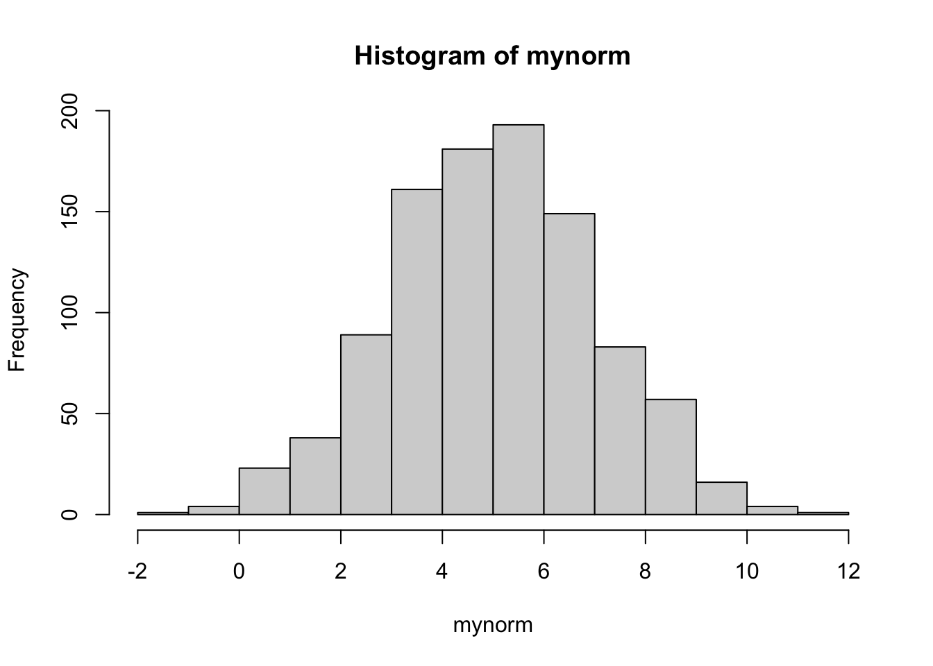

If we increase the numbers of simulated values, the histogram will more and more look like a normal distribution (bell-shaped). Now, we can look at some statistics:

mean(mynorm) #empirical mean

[1] 5.028065

var(mynorm) #empirical variance

[1] 4.025442

range(mynorm) #min, max

[1] -1.14358 11.95355

head(mynorm) #first 6 elements of the vector

[1] 5.240278 1.375246 5.303166 2.761558 5.003816 7.377037

tail(mynorm) #last 6 elements of the vector

[1] 0.7169456 6.7373514 5.6430614 3.8533123 4.4733671 4.5405532

We know assume that the 1000 values are scores from a test taken by 1000 students. We want know to compute the number of students who got a score bigger than 6. First of all we check the considered condition which returns a logical vector (remember that TRUE = 1, FALSE = 0):

mynorm > 6 # logical vector

   [1] FALSE FALSE FALSE FALSE FALSE  TRUE FALSE FALSE FALSE FALSE FALSE FALSE
  [13] FALSE FALSE FALSE FALSE  TRUE  TRUE FALSE  TRUE FALSE  TRUE  TRUE  TRUE
  [25]  TRUE  TRUE FALSE  TRUE FALSE FALSE  TRUE FALSE FALSE FALSE FALSE FALSE
  [37] FALSE FALSE FALSE  TRUE  TRUE FALSE FALSE  TRUE  TRUE  TRUE FALSE FALSE
  [49] FALSE FALSE FALSE FALSE FALSE FALSE FALSE FALSE  TRUE FALSE FALSE FALSE
  [61]  TRUE FALSE  TRUE  TRUE FALSE FALSE  TRUE FALSE FALSE FALSE FALSE FALSE
  [73] FALSE FALSE FALSE FALSE FALSE  TRUE  TRUE FALSE FALSE FALSE FALSE FALSE
  [85]  TRUE FALSE FALSE  TRUE  TRUE FALSE FALSE FALSE FALSE FALSE FALSE FALSE
  [97] FALSE  TRUE FALSE  TRUE FALSE FALSE FALSE  TRUE FALSE  TRUE FALSE  TRUE
 [109] FALSE  TRUE FALSE  TRUE  TRUE FALSE FALSE  TRUE FALSE FALSE  TRUE FALSE
 [121] FALSE FALSE  TRUE FALSE FALSE FALSE  TRUE FALSE FALSE  TRUE FALSE  TRUE
 [133]  TRUE FALSE FALSE FALSE FALSE FALSE FALSE FALSE FALSE FALSE FALSE FALSE
 [145] FALSE  TRUE  TRUE FALSE FALSE FALSE FALSE FALSE  TRUE FALSE FALSE FALSE
 [157]  TRUE FALSE FALSE  TRUE FALSE  TRUE FALSE FALSE FALSE FALSE FALSE FALSE
 [169]  TRUE FALSE FALSE FALSE FALSE FALSE FALSE FALSE  TRUE FALSE FALSE  TRUE
 [181] FALSE  TRUE FALSE FALSE FALSE  TRUE  TRUE FALSE FALSE  TRUE  TRUE FALSE
 [193] FALSE FALSE FALSE FALSE  TRUE  TRUE  TRUE FALSE FALSE  TRUE  TRUE FALSE
 [205]  TRUE  TRUE  TRUE FALSE FALSE FALSE FALSE  TRUE FALSE  TRUE  TRUE FALSE
 [217] FALSE  TRUE FALSE FALSE FALSE FALSE  TRUE FALSE  TRUE FALSE FALSE FALSE
 [229] FALSE  TRUE FALSE FALSE FALSE FALSE FALSE FALSE FALSE FALSE FALSE FALSE
 [241]  TRUE FALSE FALSE FALSE FALSE  TRUE  TRUE  TRUE FALSE  TRUE FALSE FALSE
 [253] FALSE FALSE FALSE  TRUE FALSE  TRUE  TRUE FALSE FALSE  TRUE  TRUE  TRUE
 [265] FALSE FALSE FALSE  TRUE FALSE FALSE  TRUE  TRUE FALSE  TRUE  TRUE  TRUE
 [277] FALSE FALSE FALSE  TRUE  TRUE FALSE FALSE FALSE FALSE FALSE FALSE  TRUE
 [289]  TRUE  TRUE FALSE  TRUE FALSE FALSE FALSE  TRUE FALSE FALSE FALSE FALSE
 [301] FALSE FALSE FALSE FALSE FALSE  TRUE FALSE  TRUE FALSE FALSE FALSE  TRUE
 [313] FALSE  TRUE FALSE FALSE FALSE  TRUE FALSE FALSE  TRUE FALSE  TRUE  TRUE
 [325] FALSE  TRUE  TRUE FALSE FALSE FALSE FALSE FALSE FALSE FALSE  TRUE FALSE
 [337] FALSE FALSE  TRUE FALSE FALSE FALSE  TRUE FALSE FALSE FALSE  TRUE FALSE
 [349] FALSE FALSE FALSE FALSE  TRUE FALSE FALSE  TRUE FALSE  TRUE  TRUE FALSE
 [361]  TRUE FALSE FALSE FALSE FALSE FALSE FALSE FALSE FALSE FALSE FALSE FALSE
 [373] FALSE FALSE FALSE  TRUE FALSE FALSE  TRUE FALSE FALSE  TRUE FALSE FALSE
 [385] FALSE FALSE FALSE FALSE FALSE FALSE FALSE  TRUE FALSE FALSE  TRUE  TRUE
 [397] FALSE FALSE  TRUE FALSE  TRUE  TRUE FALSE  TRUE FALSE FALSE FALSE  TRUE
 [409]  TRUE  TRUE FALSE FALSE FALSE FALSE FALSE  TRUE FALSE  TRUE  TRUE FALSE
 [421] FALSE FALSE FALSE  TRUE FALSE FALSE FALSE  TRUE FALSE FALSE FALSE FALSE
 [433] FALSE FALSE FALSE  TRUE  TRUE  TRUE  TRUE FALSE FALSE FALSE FALSE FALSE
 [445] FALSE FALSE FALSE FALSE  TRUE FALSE  TRUE FALSE FALSE FALSE FALSE FALSE
 [457] FALSE  TRUE FALSE FALSE FALSE FALSE FALSE FALSE  TRUE FALSE FALSE  TRUE
 [469]  TRUE FALSE FALSE FALSE FALSE FALSE  TRUE FALSE FALSE FALSE FALSE FALSE
 [481]  TRUE FALSE FALSE FALSE FALSE FALSE FALSE FALSE FALSE  TRUE FALSE FALSE
 [493]  TRUE  TRUE FALSE FALSE FALSE FALSE FALSE  TRUE FALSE FALSE FALSE FALSE
 [505] FALSE FALSE FALSE FALSE  TRUE FALSE FALSE  TRUE FALSE  TRUE FALSE FALSE
 [517] FALSE FALSE FALSE  TRUE FALSE FALSE FALSE  TRUE FALSE  TRUE  TRUE FALSE
 [529] FALSE FALSE FALSE FALSE FALSE FALSE  TRUE FALSE FALSE  TRUE  TRUE FALSE
 [541] FALSE  TRUE  TRUE  TRUE FALSE  TRUE FALSE FALSE FALSE FALSE FALSE FALSE
 [553] FALSE FALSE FALSE FALSE FALSE FALSE FALSE  TRUE FALSE FALSE FALSE FALSE
 [565] FALSE FALSE  TRUE  TRUE FALSE FALSE FALSE  TRUE  TRUE  TRUE FALSE  TRUE
 [577] FALSE  TRUE  TRUE  TRUE FALSE FALSE FALSE FALSE FALSE FALSE FALSE  TRUE
 [589]  TRUE FALSE FALSE FALSE FALSE FALSE FALSE FALSE  TRUE  TRUE FALSE FALSE
 [601] FALSE FALSE FALSE FALSE  TRUE  TRUE FALSE  TRUE FALSE FALSE FALSE FALSE
 [613]  TRUE  TRUE  TRUE FALSE FALSE FALSE FALSE FALSE FALSE FALSE FALSE FALSE
 [625]  TRUE FALSE FALSE FALSE  TRUE FALSE FALSE FALSE FALSE FALSE FALSE  TRUE
 [637] FALSE FALSE  TRUE FALSE  TRUE FALSE FALSE FALSE FALSE FALSE  TRUE  TRUE
 [649] FALSE FALSE FALSE FALSE  TRUE FALSE  TRUE  TRUE  TRUE FALSE FALSE FALSE
 [661]  TRUE FALSE FALSE FALSE FALSE FALSE FALSE FALSE FALSE  TRUE FALSE FALSE
 [673] FALSE  TRUE FALSE FALSE  TRUE  TRUE FALSE FALSE FALSE FALSE FALSE FALSE
 [685] FALSE FALSE FALSE FALSE FALSE FALSE FALSE  TRUE  TRUE  TRUE FALSE FALSE
 [697]  TRUE  TRUE  TRUE  TRUE  TRUE FALSE  TRUE FALSE  TRUE FALSE FALSE  TRUE
 [709] FALSE  TRUE FALSE  TRUE FALSE  TRUE  TRUE FALSE FALSE FALSE  TRUE  TRUE
 [721] FALSE FALSE FALSE  TRUE FALSE  TRUE FALSE FALSE FALSE  TRUE FALSE  TRUE
 [733] FALSE FALSE FALSE  TRUE  TRUE FALSE FALSE FALSE FALSE FALSE FALSE  TRUE
 [745]  TRUE FALSE FALSE FALSE FALSE  TRUE FALSE FALSE  TRUE FALSE FALSE  TRUE
 [757] FALSE  TRUE FALSE FALSE  TRUE FALSE FALSE  TRUE FALSE FALSE FALSE FALSE
 [769] FALSE FALSE FALSE FALSE FALSE  TRUE FALSE FALSE  TRUE FALSE FALSE FALSE
 [781] FALSE  TRUE FALSE  TRUE FALSE FALSE FALSE FALSE FALSE FALSE  TRUE  TRUE
 [793] FALSE FALSE FALSE  TRUE  TRUE FALSE FALSE FALSE  TRUE FALSE FALSE  TRUE
 [805] FALSE FALSE FALSE FALSE FALSE FALSE FALSE FALSE FALSE FALSE FALSE FALSE
 [817] FALSE FALSE FALSE FALSE  TRUE  TRUE FALSE FALSE  TRUE FALSE FALSE  TRUE
 [829]  TRUE FALSE  TRUE FALSE  TRUE  TRUE  TRUE  TRUE FALSE  TRUE FALSE  TRUE
 [841] FALSE FALSE FALSE  TRUE FALSE FALSE  TRUE FALSE  TRUE FALSE FALSE  TRUE
 [853] FALSE  TRUE FALSE FALSE FALSE FALSE  TRUE FALSE  TRUE FALSE FALSE  TRUE
 [865] FALSE  TRUE FALSE FALSE FALSE  TRUE FALSE FALSE  TRUE FALSE FALSE  TRUE
 [877]  TRUE  TRUE FALSE  TRUE FALSE  TRUE FALSE  TRUE  TRUE FALSE  TRUE  TRUE
 [889]  TRUE FALSE FALSE  TRUE  TRUE  TRUE FALSE FALSE FALSE FALSE  TRUE FALSE
 [901]  TRUE FALSE  TRUE FALSE FALSE FALSE  TRUE FALSE FALSE FALSE  TRUE FALSE
 [913]  TRUE FALSE  TRUE FALSE  TRUE FALSE FALSE FALSE FALSE FALSE  TRUE FALSE
 [925] FALSE  TRUE FALSE FALSE FALSE  TRUE FALSE FALSE  TRUE  TRUE FALSE FALSE
 [937] FALSE FALSE FALSE FALSE  TRUE  TRUE FALSE FALSE FALSE FALSE  TRUE FALSE
 [949]  TRUE FALSE FALSE FALSE FALSE FALSE  TRUE  TRUE FALSE FALSE  TRUE FALSE
 [961]  TRUE FALSE FALSE  TRUE FALSE  TRUE  TRUE  TRUE FALSE FALSE  TRUE FALSE
 [973] FALSE  TRUE FALSE  TRUE FALSE FALSE  TRUE FALSE FALSE  TRUE FALSE  TRUE
 [985]  TRUE FALSE FALSE  TRUE FALSE FALSE FALSE  TRUE  TRUE FALSE FALSE  TRUE
 [997] FALSE FALSE FALSE FALSE

If we sum the elements in the logical vector we will basically compute the number of times the condition is met:

sum(mynorm > 6) #absolute frequency

[1] 310

To get the corresponding percentage we will use the mean function instead of sum:

mean(mynorm > 6) * 100 #percentage

[1] 31

To sum up, the number of students that gets more than 6 in the test score are 310, that in percentage is the 31% of the total.

We are now interested in computing the % of scores between 3 and 6. In this case we have two conditions that should be jointly satisfied; thus we need the AND operator which is implemented in R with &:

mean(mynorm > 3 & mynorm < 6) * 100

[1] 53.5

We can observe that the majority of the observation are around the mean.

If instead we want to compute the % of scores lower than 0 OR bigger than 10 we will use the | operator:

#logical operator
mynorm <0 | mynorm > 10

   [1] FALSE FALSE FALSE FALSE FALSE FALSE FALSE FALSE FALSE FALSE FALSE FALSE
  [13] FALSE FALSE FALSE FALSE FALSE FALSE FALSE FALSE FALSE FALSE FALSE FALSE
  [25] FALSE FALSE FALSE FALSE FALSE FALSE FALSE FALSE FALSE FALSE FALSE FALSE
  [37] FALSE FALSE FALSE FALSE FALSE FALSE FALSE FALSE FALSE FALSE FALSE FALSE
  [49] FALSE FALSE FALSE FALSE FALSE FALSE FALSE FALSE FALSE FALSE FALSE FALSE
  [61] FALSE FALSE FALSE FALSE FALSE FALSE FALSE FALSE FALSE FALSE FALSE FALSE
  [73] FALSE FALSE FALSE FALSE FALSE FALSE FALSE FALSE FALSE FALSE FALSE FALSE
  [85] FALSE FALSE FALSE FALSE FALSE FALSE FALSE FALSE FALSE FALSE FALSE FALSE
  [97] FALSE FALSE FALSE FALSE FALSE FALSE FALSE FALSE FALSE FALSE FALSE FALSE
 [109] FALSE FALSE FALSE FALSE FALSE FALSE FALSE FALSE FALSE FALSE FALSE FALSE
 [121] FALSE FALSE FALSE FALSE FALSE FALSE FALSE FALSE FALSE FALSE FALSE FALSE
 [133] FALSE FALSE FALSE FALSE FALSE FALSE FALSE FALSE FALSE FALSE FALSE FALSE
 [145] FALSE FALSE FALSE FALSE FALSE FALSE FALSE FALSE FALSE FALSE FALSE FALSE
 [157] FALSE FALSE FALSE  TRUE FALSE FALSE FALSE FALSE FALSE FALSE FALSE FALSE
 [169] FALSE FALSE FALSE FALSE FALSE FALSE FALSE FALSE FALSE FALSE FALSE FALSE
 [181] FALSE FALSE FALSE FALSE FALSE FALSE FALSE FALSE FALSE FALSE FALSE FALSE
 [193] FALSE FALSE FALSE FALSE FALSE FALSE FALSE FALSE FALSE FALSE FALSE FALSE
 [205] FALSE FALSE FALSE FALSE FALSE FALSE FALSE FALSE FALSE FALSE FALSE FALSE
 [217]  TRUE FALSE FALSE FALSE FALSE FALSE FALSE FALSE FALSE FALSE FALSE FALSE
 [229] FALSE FALSE FALSE FALSE FALSE FALSE FALSE FALSE FALSE FALSE FALSE FALSE
 [241] FALSE FALSE FALSE FALSE FALSE FALSE FALSE FALSE FALSE FALSE FALSE FALSE
 [253] FALSE FALSE FALSE FALSE FALSE FALSE FALSE FALSE FALSE FALSE FALSE FALSE
 [265] FALSE FALSE FALSE FALSE FALSE FALSE FALSE FALSE FALSE FALSE FALSE FALSE
 [277] FALSE FALSE FALSE FALSE FALSE FALSE FALSE FALSE FALSE FALSE FALSE FALSE
 [289] FALSE FALSE FALSE FALSE FALSE FALSE FALSE FALSE FALSE FALSE FALSE FALSE
 [301] FALSE FALSE FALSE FALSE FALSE FALSE FALSE FALSE FALSE FALSE FALSE FALSE
 [313] FALSE FALSE FALSE FALSE FALSE FALSE FALSE FALSE FALSE FALSE FALSE FALSE
 [325] FALSE FALSE  TRUE FALSE FALSE FALSE FALSE FALSE FALSE FALSE FALSE FALSE
 [337] FALSE FALSE FALSE FALSE FALSE FALSE FALSE FALSE FALSE  TRUE FALSE FALSE
 [349] FALSE FALSE FALSE FALSE FALSE FALSE FALSE FALSE FALSE FALSE FALSE FALSE
 [361] FALSE FALSE FALSE FALSE FALSE FALSE FALSE FALSE FALSE FALSE FALSE FALSE
 [373] FALSE FALSE FALSE FALSE FALSE FALSE FALSE FALSE FALSE FALSE FALSE FALSE
 [385] FALSE FALSE FALSE FALSE FALSE FALSE FALSE FALSE FALSE FALSE FALSE FALSE
 [397] FALSE FALSE FALSE FALSE FALSE FALSE FALSE FALSE FALSE FALSE FALSE FALSE
 [409] FALSE FALSE FALSE FALSE FALSE FALSE FALSE FALSE FALSE FALSE FALSE FALSE
 [421] FALSE FALSE FALSE FALSE FALSE FALSE FALSE FALSE FALSE FALSE FALSE FALSE
 [433] FALSE FALSE  TRUE FALSE FALSE FALSE FALSE FALSE FALSE FALSE FALSE FALSE
 [445] FALSE FALSE FALSE FALSE FALSE FALSE FALSE FALSE FALSE FALSE FALSE FALSE
 [457] FALSE FALSE FALSE FALSE FALSE FALSE FALSE FALSE FALSE FALSE FALSE FALSE
 [469] FALSE FALSE FALSE FALSE FALSE FALSE FALSE FALSE FALSE FALSE FALSE FALSE
 [481] FALSE FALSE FALSE FALSE FALSE FALSE FALSE FALSE FALSE FALSE FALSE  TRUE
 [493] FALSE FALSE FALSE FALSE FALSE FALSE FALSE FALSE FALSE FALSE FALSE FALSE
 [505] FALSE FALSE FALSE FALSE FALSE FALSE FALSE FALSE FALSE FALSE FALSE FALSE
 [517] FALSE FALSE FALSE FALSE FALSE FALSE FALSE FALSE FALSE FALSE FALSE FALSE
 [529] FALSE FALSE FALSE FALSE FALSE FALSE FALSE FALSE FALSE FALSE FALSE FALSE
 [541] FALSE FALSE FALSE FALSE FALSE FALSE FALSE FALSE FALSE FALSE FALSE FALSE
 [553] FALSE FALSE FALSE FALSE FALSE FALSE FALSE FALSE FALSE FALSE FALSE FALSE
 [565]  TRUE FALSE FALSE FALSE FALSE FALSE FALSE FALSE FALSE FALSE FALSE FALSE
 [577] FALSE FALSE FALSE FALSE FALSE FALSE FALSE FALSE FALSE FALSE FALSE FALSE
 [589] FALSE FALSE FALSE FALSE FALSE FALSE FALSE FALSE FALSE FALSE FALSE FALSE
 [601] FALSE FALSE FALSE FALSE FALSE FALSE FALSE FALSE FALSE FALSE FALSE FALSE
 [613] FALSE FALSE FALSE FALSE FALSE FALSE FALSE FALSE FALSE FALSE FALSE FALSE
 [625] FALSE FALSE FALSE FALSE FALSE FALSE FALSE FALSE FALSE FALSE FALSE FALSE
 [637] FALSE FALSE FALSE FALSE FALSE FALSE FALSE FALSE FALSE FALSE FALSE FALSE
 [649] FALSE FALSE FALSE FALSE FALSE FALSE FALSE FALSE FALSE FALSE FALSE FALSE
 [661] FALSE FALSE FALSE FALSE FALSE FALSE FALSE FALSE FALSE FALSE FALSE FALSE
 [673] FALSE FALSE FALSE FALSE FALSE FALSE FALSE FALSE FALSE FALSE FALSE FALSE
 [685] FALSE FALSE FALSE FALSE FALSE FALSE FALSE FALSE FALSE FALSE FALSE FALSE
 [697] FALSE FALSE FALSE FALSE FALSE FALSE FALSE FALSE FALSE FALSE FALSE FALSE
 [709] FALSE FALSE FALSE FALSE FALSE FALSE FALSE FALSE FALSE FALSE FALSE FALSE
 [721] FALSE FALSE FALSE FALSE FALSE FALSE FALSE FALSE FALSE FALSE FALSE FALSE
 [733] FALSE FALSE FALSE FALSE FALSE FALSE FALSE FALSE FALSE FALSE FALSE FALSE
 [745] FALSE FALSE FALSE FALSE FALSE FALSE FALSE FALSE FALSE FALSE FALSE FALSE
 [757] FALSE FALSE FALSE FALSE FALSE FALSE FALSE FALSE FALSE FALSE FALSE FALSE
 [769] FALSE FALSE FALSE FALSE FALSE  TRUE FALSE FALSE  TRUE FALSE FALSE FALSE
 [781] FALSE FALSE FALSE FALSE FALSE FALSE FALSE FALSE FALSE FALSE FALSE FALSE
 [793] FALSE FALSE FALSE FALSE FALSE FALSE FALSE FALSE FALSE FALSE FALSE FALSE
 [805] FALSE FALSE FALSE FALSE FALSE FALSE FALSE FALSE FALSE FALSE FALSE FALSE
 [817] FALSE FALSE FALSE FALSE FALSE FALSE FALSE FALSE FALSE FALSE FALSE FALSE
 [829] FALSE FALSE FALSE FALSE FALSE FALSE FALSE FALSE FALSE FALSE FALSE FALSE
 [841] FALSE FALSE FALSE FALSE FALSE FALSE FALSE FALSE FALSE FALSE FALSE FALSE
 [853] FALSE FALSE FALSE FALSE FALSE FALSE FALSE FALSE FALSE FALSE FALSE FALSE
 [865] FALSE FALSE FALSE FALSE FALSE FALSE FALSE FALSE FALSE FALSE FALSE FALSE
 [877] FALSE FALSE FALSE FALSE FALSE FALSE FALSE FALSE FALSE FALSE FALSE FALSE
 [889] FALSE FALSE FALSE FALSE FALSE FALSE FALSE FALSE FALSE FALSE FALSE FALSE
 [901] FALSE FALSE FALSE FALSE FALSE FALSE FALSE FALSE FALSE FALSE FALSE FALSE
 [913] FALSE FALSE FALSE FALSE FALSE FALSE FALSE FALSE FALSE FALSE FALSE FALSE
 [925] FALSE FALSE FALSE FALSE FALSE FALSE FALSE FALSE FALSE FALSE FALSE FALSE
 [937] FALSE FALSE FALSE FALSE FALSE FALSE FALSE FALSE FALSE FALSE FALSE FALSE
 [949] FALSE FALSE FALSE FALSE FALSE FALSE FALSE FALSE FALSE FALSE FALSE FALSE
 [961] FALSE FALSE FALSE FALSE FALSE FALSE FALSE FALSE FALSE FALSE FALSE FALSE
 [973] FALSE FALSE FALSE FALSE FALSE FALSE FALSE FALSE FALSE FALSE FALSE FALSE
 [985] FALSE FALSE FALSE FALSE FALSE FALSE FALSE  TRUE FALSE FALSE FALSE FALSE
 [997] FALSE FALSE FALSE FALSE

#absolute value
sum(mynorm <0 | mynorm >10)

[1] 10

#proportion
mean(mynorm <0 | mynorm >10)

[1] 0.01

#percentage
mean(mynorm < 0 | mynorm > 10) * 100

[1] 1

Moving to the tails of the distribution, we observe a small number of observations.

Finally remember that you can use the summary function to get some summary statistics about your vector:

summary(mynorm)

   Min. 1st Qu.  Median    Mean 3rd Qu.    Max. 
 -1.144   3.616   5.035   5.028   6.367  11.954

2.5 Exercises Lecture 1

2.5.1 Exercise 1

Compute \(\exp(3-\frac{4}{5})+\frac{\sqrt{3+2^5}}{4-7\cdot \log(10))}\)

exp(3-4/5) + sqrt(3+2^5)/(4-7*log(10))

[1] 8.536811

Create the vector named x which contains the following values \((10, log(0.2), 6/7, exp(4), sqrt(54), -0.124)\):

x=c(10, log(0.2), 6/7, exp(4), sqrt(54), -0.124)
x

[1] 10.0000000 -1.6094379  0.8571429 54.5981500  7.3484692 -0.1240000

Find the length of x.

length(x)

[1] 6

Which elements of x are between 0 (included) AND 1 (excluded)? Hint: the AND operator is given by &. Compute also the corresponding absolute (count) and relative frequency (proportions).

x >= 0 & x<1

[1] FALSE FALSE  TRUE FALSE FALSE FALSE

sum (x >= 0 & x<1)

[1] 1

mean (x >= 0 & x<1)

[1] 0.1666667

Which elements of x are negative? Substitute them with the same number in absolute value.

x[x<= 0] = abs(x[x<= 0])

Extract from x the 2nd and 4th value and save them in a new vector named y. Compute \(y+sqrt(exp(-0.4))\).

y=x[c(2,4)]
y

[1]  1.609438 54.598150

y+sqrt(exp(-0.4))

[1]  2.428169 55.416881

2.5.2 Exercise 2

Read the help pages of the functions sample and seq.

#?sample
#?seq

Run the following lines of code and try to understand what it is going on.

#Attention: we set the seed in order to work with the same data
set.seed(2233)
xVec = sample(seq(0,999), 25, replace=T)
xVec

 [1] 513 773 693 506 706 208 111 713 816 773 465 661 561 883 871 158 498  91  95
[20]  94 685 564 833 746 425

set.seed(3344)
yVec = sample(seq(0,999, length=100), 25, replace=F)
yVec

 [1] 908.18182 888.00000 999.00000  40.36364 433.90909 938.45455 615.54545
 [8] 898.09091 363.27273 817.36364 736.63636 494.45455 242.18182 948.54545
[15] 302.72727 181.63636 807.27273 555.00000 353.18182 464.18182 797.18182
[22] 222.00000 766.90909 988.90909 696.27273

set.seed(33)
zVec = sample(seq(0,999, by=10), 5, replace=F)
zVec

[1] 410  70 850 590  80

Compute some summary statistics for the three vectors.

summary(xVec)

   Min. 1st Qu.  Median    Mean 3rd Qu.    Max. 
   91.0   425.0   564.0   537.7   746.0   883.0

summary(yVec)

   Min. 1st Qu.  Median    Mean 3rd Qu.    Max. 
  40.36  363.27  696.27  618.37  888.00  999.00

summary(zVec)

   Min. 1st Qu.  Median    Mean 3rd Qu.    Max. 
     70      80     410     400     590     850

Select the values in yVec which are bigger than 600.

xVec[yVec>600]

 [1] 513 773 693 208 111 713 773 465 883 498 685 833 746 425

Select the values in yVec which are between 600 and 800 and save them in a new vector called yVec_sel1. Pick out the values in yVec which are bigger than 600 or lower than 800 and save them in a new vector called yVec_sel2. Which is the length of yVec_sel1 and yVec_sel2?

yVec_sel1= yVec[yVec>600 & yVec<800]
yVec_sel1

[1] 615.5455 736.6364 797.1818 766.9091 696.2727

length(yVec_sel1)

[1] 5

yVec_sel2= yVec[yVec>600 | yVec<800]
yVec_sel2

 [1] 908.18182 888.00000 999.00000  40.36364 433.90909 938.45455 615.54545
 [8] 898.09091 363.27273 817.36364 736.63636 494.45455 242.18182 948.54545
[15] 302.72727 181.63636 807.27273 555.00000 353.18182 464.18182 797.18182
[22] 222.00000 766.90909 988.90909 696.27273

length(yVec_sel2)

[1] 25

Which are the values in xVec that have the same position of the values in yVec which are bigger than 600?

xVec[yVec>600]

 [1] 513 773 693 208 111 713 773 465 883 498 685 833 746 425

Compute the sum and the difference of the first 5 elements of the 2 vectors. Hint: to index the first 5 elements you can use 1:5.

(xVec + yVec)[1:5]

[1] 1421.1818 1661.0000 1692.0000  546.3636 1139.9091

# or 
xVec[1:5] + yVec[1:5]

[1] 1421.1818 1661.0000 1692.0000  546.3636 1139.9091

xVec[1:5] - yVec[1:5]

[1] -395.1818 -115.0000 -306.0000  465.6364  272.0909

# or 
(xVec - yVec)[1:5]

[1] -395.1818 -115.0000 -306.0000  465.6364  272.0909

For xVec compute the following formula \(\frac{\sum_{i=1}^n (x_i-\bar x)^2}{n}\), where \(n\) is the vector length and \(\bar x\) is the vector mean. Is the result equal to the one obtained with var? Why?

sum((xVec-mean(xVec))^2)/length(xVec)

[1] 68756.86

var(xVec) #this is computed with n-1

[1] 71621.73

sum((xVec-mean(xVec))^2)/(length(xVec)-1)

[1] 71621.73

For xVec compute the following formula \(\frac{\sum_{i=1}^n |x_i-Me|}{n}\), where \(n\) is the vector length and \(Me\) is the vector median.

sum(abs(xVec-median(xVec)))/length(xVec)

[1] 217.12

Consider zVec. Try to understand how the functions sort and order work when applied to zVec. Check also their help pages.

sort(zVec)

[1]  70  80 410 590 850

order(zVec)

[1] 2 5 1 4 3

zVec[order(zVec)]

[1]  70  80 410 590 850

2.5.3 Exercise 3

Simulate a vector (named x) of 50 values from the Uniform distribution defined between 2 and 6. Use 33 as seed.

set.seed(33)
x = runif(50, min = 2, max = 6)
x

 [1] 3.783762 3.578601 3.934915 5.675504 5.375526 4.069398 3.748500 3.372793
 [9] 2.062068 2.471965 4.763944 3.041943 2.900205 3.369545 5.127552 5.372987
[17] 5.098995 3.548772 2.543060 5.601430 4.265811 2.170937 3.953277 3.404893
[25] 5.878647 5.158316 4.386521 3.426682 5.034833 3.044203 3.975928 5.171593
[33] 3.771996 3.333062 4.503074 2.544773 4.194731 5.687327 3.104135 5.669656
[41] 3.316407 2.564976 4.457138 3.524313 5.061443 5.356332 4.708356 2.568770
[49] 4.293707 5.715988

Compute the mean of the simulated values. Moreover, compute the percentage of values between 4 and 5.

mean(x)

[1] 4.073786

mean(x > 4 & x < 5)*100

[1] 18

Substitute the values bigger than 5 with values simulated from the Uniform(0,1) distribution. Use 11 as seed. Then recompute again the mean of the vector.

set.seed(11)
sum(x>5) #15 values

[1] 15

x[x > 5] = runif(sum(x>5))
x

 [1] 3.7837619167 3.5786012439 3.9349154988 0.2772497942 0.0005183129
 [6] 4.0693984665 3.7485000174 3.3727928633 2.0620678402 2.4719646480
[11] 4.7639435958 3.0419427389 2.9002048206 3.3695448926 0.5106083730
[16] 0.0140479084 0.0646897766 3.5487719383 2.5430602795 0.9548492255
[21] 4.2658106284 2.1709366413 3.9532770133 3.4048928861 0.0864958912
[26] 0.2899750092 4.3865210470 3.4266821351 0.8806991728 3.0442030625
[31] 3.9759276798 0.1232162013 3.7719958415 3.3330622222 4.5030738572
[36] 2.5447727554 4.1947311088 0.1751129227 3.1041345717 0.4407502718
[41] 3.3164071562 2.5649762955 4.4571379730 3.5243129777 0.9071829736
[46] 0.8510418669 4.7083558943 2.5687704161 4.2937068893 0.7339874927

mean(x)

[1] 2.580272